This is a continuation of a 2 part series in predicting the products of a chemical reaction using deep learning methods. Checkout the first part here.

In part 1, we:

1. First introduced the problem statement
2. Then we saw how a molecule is represented in a graph network
3. Next we looked into the node and edge features and how they’re calculated
4. And finally, briefly looked into how Coley et al. structured the problem to make the final prediction

In this blog, we’ll jump into the inner working of the GCN model and see how the model actually work.

Predicting the reactive sites

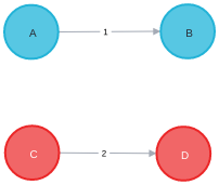
A chemical reaction, in this problem, is interpreted as a set of changes in bond order in a collection of reactant molecules. In other words, all the reactants and reagents for a reaction are treated as one big graph. Break some bonds, form some bonds: The resultant state of the graph is products. Confused? Okay, let’s look at an example. Consider the following reaction:

AB + CD 🠒 AD + CB

And, the reactant graph is represented as below. There are single bonds between the pairs (A, B), and (C, D) and 0 bonds (no bond) between the pair of (A, C), (A, D), (B, C), and (B, D).

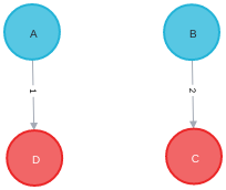
After passing through the trained model, the model predicts that the bond between the pairs (A, B) and (C, D) breaks, and the pairs (A, D) and (B, C) forms a single bond each. The pairs (A, C) and (B, D) remains unchanged (no bond). The resultant graph will look like this:

To predict these bond changes, the authors have used the Weisfeiler-Lehman Network (WLN), a type of graph convolutional neural network. See the below figure for the WLN workflow.

Initially, the atoms and bonds are featurized as per the rules we discussed earlier. Then a local embedding iteratively updates the atom-level representation by incorporating the features of the atoms around it. This is done to capture the neighborhood of the atom (an atom’s behavior is also influenced by the type of atoms that surrounds it).

The step B in the following figure illusterates this by taking the example of atom v. It has 4 neighbors: u, x, y, and w. First, the feature vectors for these neighbors (f_u, f_x, f_y, and f_w), along with the connectivity information on how these are connected with atom v (f_uv, f_xv, f_yv, and f_wv) are passed through a feed-forward neural network to obtain a single feature vector representation for the neighbors (let’s call it f_nbr). Then, this obtained vector (f_nbr), along with the atom v’s feature vector (f_v) is passed through another feed-forward neural network to obtain a new representation for the atom, f_{v, updated}. This process is repeated multiple times for each atom and the generated features are termed as local features (c_v).

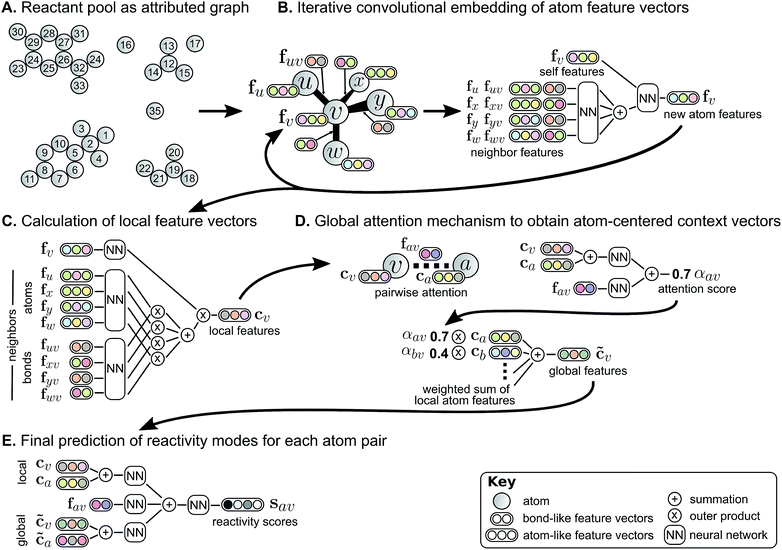
Intuitively explaining, each atom is updating its features as per its neighbors, which in turn are updating their features as per their neighbors, which are again doing the same thing. So the atom v in question is not only looking at its immediate neighbors but also the atoms a few hops away from it. Although, this raises one big question: how do you account for the interaction of reactants with the solvents or catalysts? The atoms in the solvent are completely disconnected from the reactants and hence their feature information will never reach the reactant atom features and vice-versa. This is a problem because both solvents and catalysts are an integral part of a reaction.

To deal with this problem, a global attention mechanism is implemented where all atoms in the reactant graph attend to (“look at”) all other atoms. Now, do all atoms contribute equally to the behavior of an atom in question? Of course not. Some atoms may be far more impactful than others. An attention score is generated for each of the atoms that effectively tells us the importance of the atom in the behavior of the central atom. For example, in step D in the above figure, atom v is the central atom and the impact of the atom a is displayed by generating an attention score (α_av). A high value of α_av means that atom a plays a very crucial role in the behavior of the atom v. A global context vector for each atom is generated based on contributions from the representations of all atoms weighted by the strength of this attention. This global feature vector is termed as a context vector (c̃_v).

Finally, pairwise sums of these learned atom-level representations, both from the local atomic environment (c_v) and from the influence of all other species (c̃_v), are used to calculate the likelihood scores. The model is trained to assign a score to each pair of atoms signifying their tendency to form or break a bond (step E).

Enumerating the product candidates

The authors have structured the problem in such a way that the model assigns a score to all possible pairs of atoms. But the model is not perfect and hence won’t be assigning a perfect 0 score to any of the pairs. That also means that there are going to as many bond changes predicted as many there are pairs of atoms (ⁿC₂ pairs if there are n atoms in the reactant graph). And total 2^nC₂ total candidates for products. Clearly, that’s far too many. To avoid this explosion of candidates, the authors limit the enumeration by picking only the K most likely bond changes. The value of K can be tuned to decide between coverage of true products versus computational restrictions (a higher value of K ensures higher chances of not missing the true product of that reaction). Further, a preliminary analysis of the dataset by the author revealed that the majority of reactions had undergone at most 5 bond changes to form the products. This limitation is applied here to further reduce the number of candidates. Therefore, the number of candidates is bounded by:

Also, many of the candidates violate the valence rule so valence and connectivity constraints substantially reduce the number of valid candidates produced by this enumeration.

Ranking the candidates to get the final product

Once all possible candidates are decided, the final step is to rank them and decide the final product. In their previous approaches (1, 2), the authors had treated this step as a separate task itself. And it does seem like a separate task as it’s concerned with ranking a set of candidates. It doesn’t matter if these candidates came from the output of the previous model or experienced scientists created it manually.

However, the authors claim that this approach fails to utilize a key aspect of the enumeration step: candidate outcomes produced by combinations of more likely bond changes are themselves more likely to be the true outcome. The quantitative scores for each bond change when perceiving likely modes of reactivity provides an initial ranking of candidate reaction outcomes. The remaining evaluation task serves to refine these preliminary rankings, now taking into account the likelihood of each set of bond changes.

Weisfeiler-Lehman Difference Networks (WLDNs) which are conceptually similar to the WLN are used for this ranking. The previous model was taking a reactant graph as input but this time the candidates are also embedded as attributed graphs along with the reactants to obtain a local atom-level representation. This is the idea here: For each candidate, we’ll have a reaction. One (or more in case there is a side reaction) of them is the correct reaction and the rest false. Now, the task is to decide which one is right.

To do this, the authors, first, calculate a numerical representation of each reaction. This representation is calculated by subtracting the atom representations of the reactants from the candidates (The authors claim that this so that the model can focus on the key difference between the reactants r and products p, while also incorporating the necessary chemical contexts surrounding the changes. In other words, an atom v’s feature vector should deviate from zero only if it is close to the reaction center, thus focusing the processing on the reaction center and its immediate context). Then, after passing this fingerprint through a feed-forward neural network, the output is added to the preliminary score obtained by summing the bond change likelihoods as perceived by the WLN. The reaction with the highest resultant score is termed as the main reaction and the corresponding candidates as the main products.

Results

On the dataset the authors used, the models were able to predict the correct products 85.6% of the time which the authors claim to be a substantial improvement over previous state-of-the-art models. This accuracy went up to 90.5% for top-2, 92.8% for top-3 and 93.4% for top-5 predictions. Here, 93.4% for top-5 prediction means that 93.4% of the time, the true products were among the top 5 predictions made by the model.

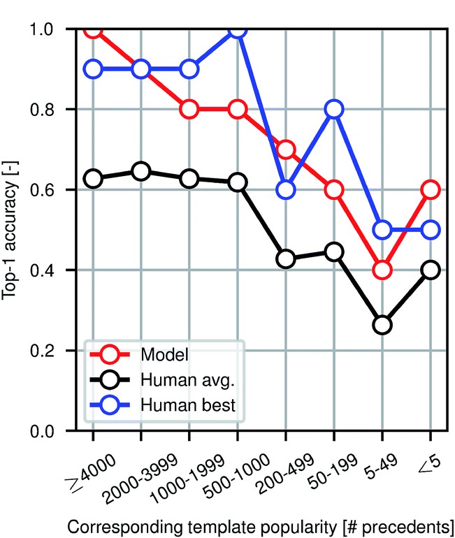
To evaluate the performance of the model against human experts, the authors conducted a small-scale experiment where they asked a team of participants to find the products of a set of 80 reactions. Among the participants were chemistry and chemical engineering graduate students, postdocs, and professors. The following figure illustrates the popularity of the reaction template used versus different evaluators. It is evident that the model performs at the level of an expert chemist for this prediction task.

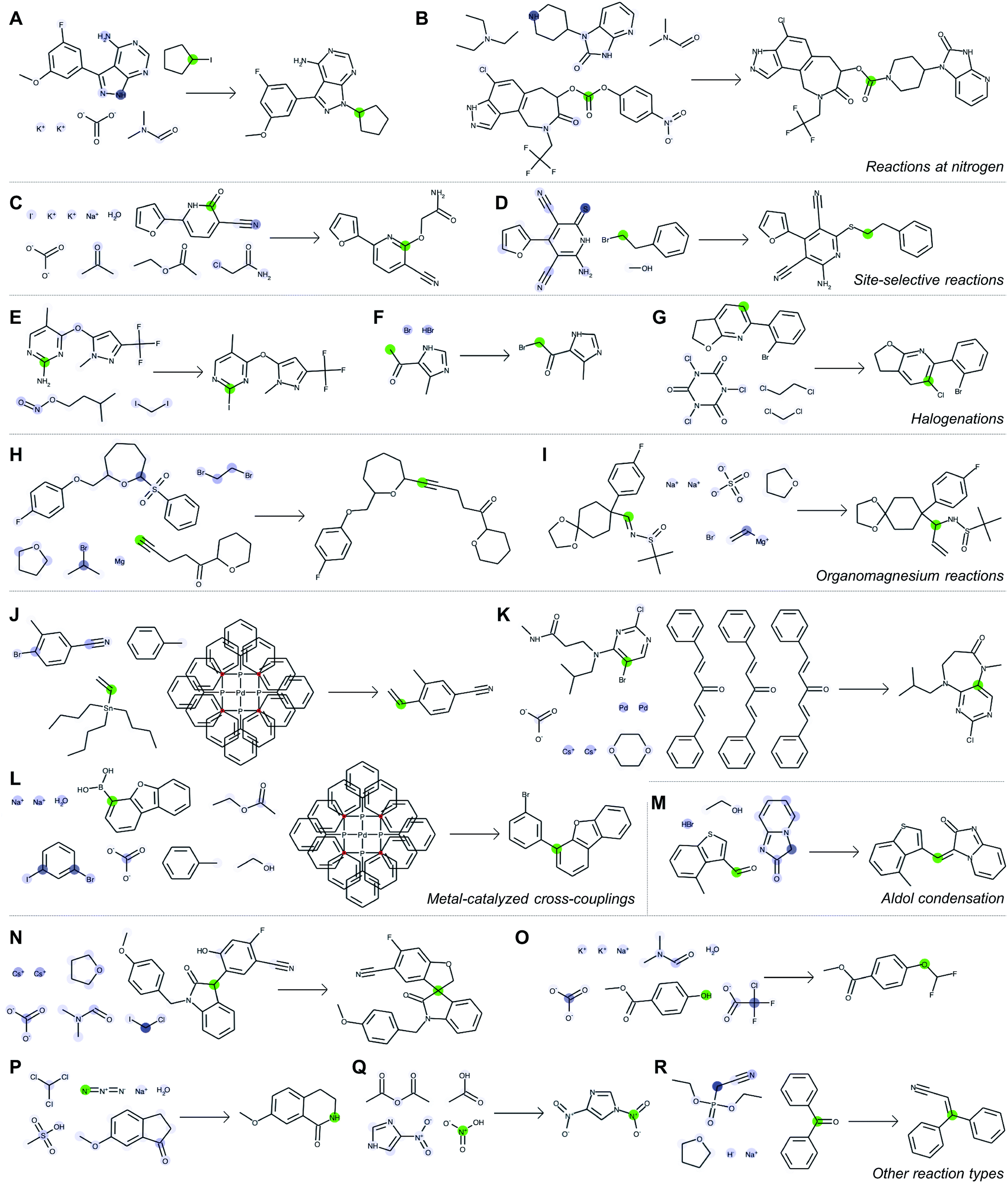
Examples

Now we know all about the model and the process of making the predictions, let’s see some examples of the actual predictions. The following diagram illustrates a few such samples. For each of the reactions, the authors selected an atom (highlighted in green) and showcased the influence of other atoms on its behavior. A darker blue color means higher influence.

Observations

Before we wrap up this article, there are a few things that are worth noting:

1. The majority of the reactions in the dataset undergo at most 5 bond changes. It would be interesting to see how the model performs on more complex reactions involving more than 5 bond changes.
2. The algorithm hasn’t taken into account the reaction conditions such as the temperature of the system. The physical conditions can significantly change the reaction outcome.
3. The human benchmarking experiment conducted by the authors uses only 80 reactions which is a very small number compared to the size of the dataset used. Hence, comparison of algorithm accuracy against human experts requires further exploration.
4. The model does not comment on the product yield and the time taken for the completion of the reaction.

Conclusion

This approach by the authors not only proves the applications of machine learning in chemistry but also implies that a deep learning algorithm need not be a black box which is often the case in this field. By using the color mechanism to highlight the atoms (green and blue), the authors have shown that the model can be interpreted to show what it actually learned.

References and Further Reading

• Coley, Connor W.; Jin, Wengong; Rogers, Luke; Jamison, Timothy F.; S Jaakkola, Tommi; Green, William H.; et al. (2018): A Graph-Convolutional Neural Network Model for the Prediction of Chemical Reactivity.
• Python and TensorFlow implementation of this paper is available here.