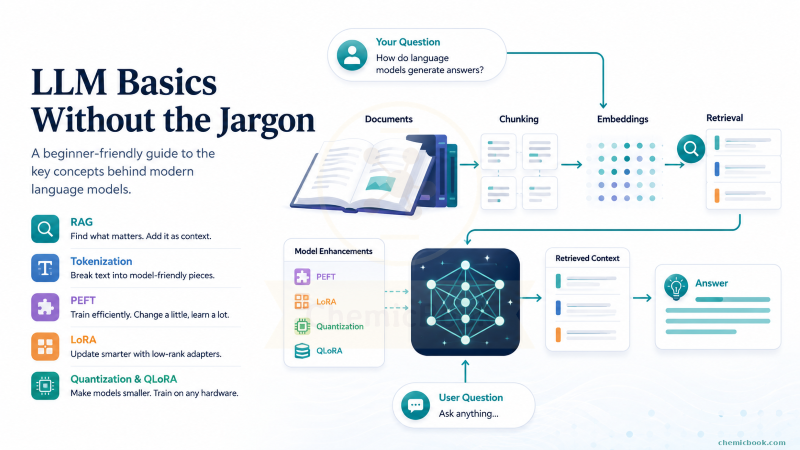
Everyone talks about LLMs, but the real magic is often in the pieces around them: tokens, embeddings, retrieval, adapters, and compressed weights. This post gently opens the black box and shows how these ideas fit together to power the AI tools we use every day - without drowning you in jargon.

Table of Contents

• Retrieval Augmented Generation (RAG)
  • Introduction
  • Context
  • Chunking
  • Embeddings
  • Vector Databases
  • Wrapping up
• Tokens and Tokenization
• LLM Finetuning Terminology
  • Parameter-Efficient Fine-Tuning (PEFT)
  • Low-Rank Adaptation (LoRA)
  • Quantization
  • Quantized Low-Rank Adaptation (QLoRA)
• Final Wrap-up

Retrieval Augmented Generation (RAG)

Introduction

Let’s say I ask ChatGPT: “What does Tolkien say about people who wander?”. If the relevant passage is not available to the model, it may give a vague answer or say that it needs more information.

Now let’s say I provide a short passage first and then ask the same question. For example:

Here is a short passage from The Lord of the Rings:

"Not all those who wander are lost."

What does the passage say about people who wander?

Because I have provided the relevant passage, the chatbot can answer more directly this time (Augmented Generation). This additional detail is called Context.

Context

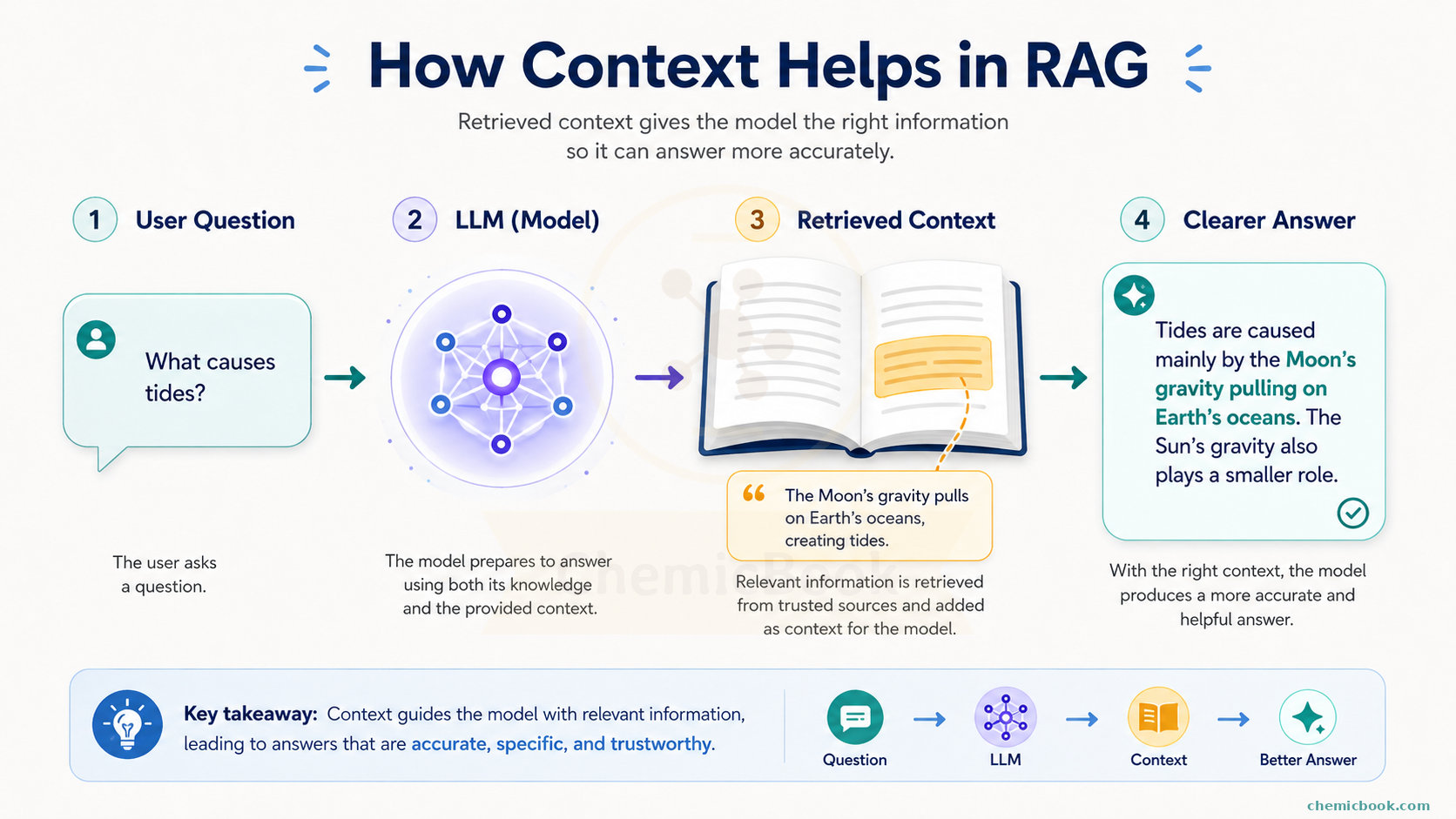
Let’s say a new book is published which ChatGPT has never seen and we want to ask some questions about it. One method we already discussed is to copy and paste the entire book as context and then ask the question at the end. But this method has two major issues.

1. Context Length: Every LLM has a limit on how long the input can be. For example, older GPT-4 had a limit of about 8k tokens (we’ll see what’s a token in a minute). So if the book has many pages, it might not fit in the context and we’ll get an error.

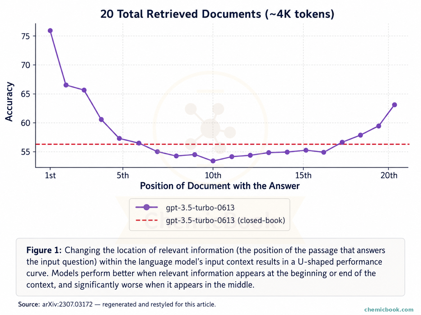
2. Finding a needle in a haystack: Even if it does fit in the context, there’s no guarantee that the chatbot will be able to find the right answer due to large amount of information available in the context. The below chart shows that the models can struggle to use relevant information in long contexts, especially when it appears in the middle.

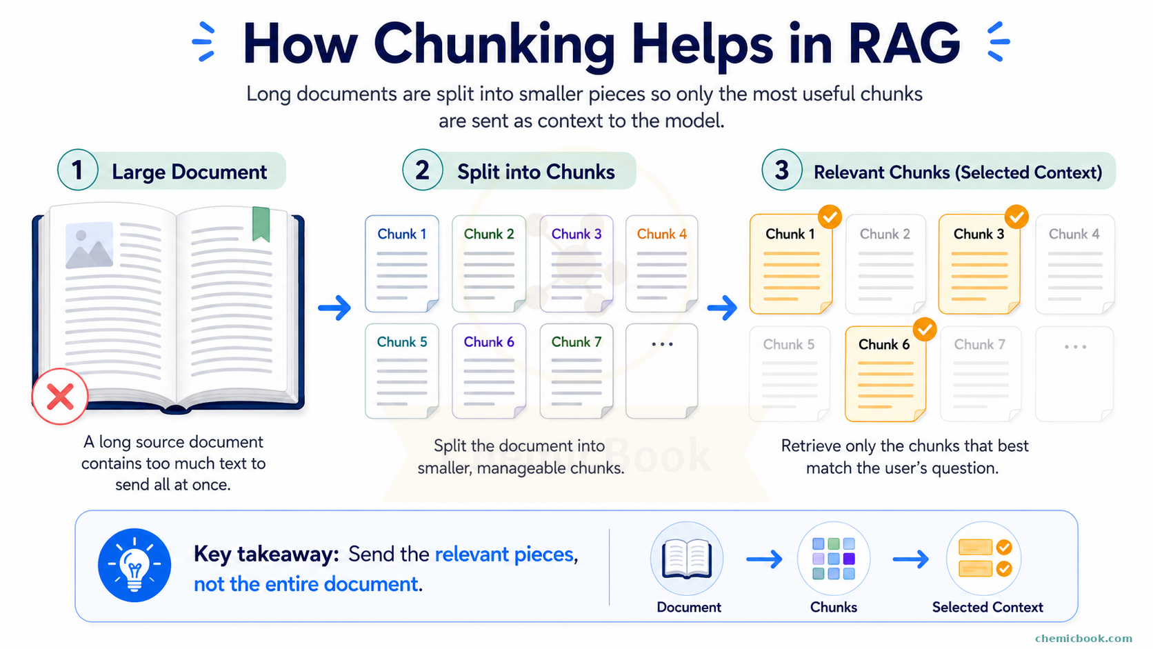
So passing the complete context in one go is not enough. We need a better way. What if, instead of passing the entire book as context, we find a shorter chunk of text containing the answer and pass it as context?

Chunking

Chunking is the process of splitting a long piece of text into smaller chunks and then only passing the relevant chunks as context. This approach solves both the issues: context length is reduced and amount of information is also reduced so that the LLM can focus more on relevant details.

There are many ways to split a text and the right method depends on the user and problem you’re trying to solve. For example, you can split a long book by chapters, sections, paragraphs, or even sentences. Each of these methods has its own advantages and can be chosen based on the context of the task at hand. Some of the common methods of chunking are:

1. Fixed Size Chunking: This is the most crude and simplest method of segmenting the text. It breaks down the text into chunks of a specified number of characters, regardless of their content or structure. For example, you splitting a text by keeping a maximum of 500 characters in each chunk.

2. Recursive Chunking: This method recursively splits the text into chunks until a desired context size is achieved. For example, it can first try to split a text by paragraphs. If any paragraph is still too long, it can further split it by lines or any other method defined by the user.

3. Document-specific Chunking: Each document has its own structure. Rather than using a fixed number of characters or a recursive process, this method creates chunks that align with the logical sections of the document, like paragraphs or subsections. For example, if the document contains programming code, it makes sense to ensure that functions or classes are not split in between chunks.

There are other methods like Semantic chunking, token-based chunking, agent-based chunking, etc. You can even write your own functions to define the right approach.

Coming back to the original problem, we wanted to split the book into smaller chunks and only pass the relevant chunks as context. You might notice an immediate issue here: How do we find the right chunks to use as the context? Because, if we already knew where the answer is in the book, we might not even need the chatbot. To understand this, we first need to understand the concept of Embeddings.

Embeddings

Embeddings are a way to represent pieces of text (like words, sentences, or even whole documents) as numerical vectors. These vectors capture the meaning and context of the text in a form that a machine can understand. Think of embeddings as a way to translate words and phrases into a language that computers can use to find patterns and make predictions.

Suppose we have a small vocabulary of words: [“cat,” “dog,” “space,” “rocket”]. Each word is assigned a unique vector of numbers. For instance:

• “cat” → [0.1, 0.3, 0.5]
• “dog” → [0.2, 0.4, 0.6]
• “space” → [0.7, 0.8, 0.9]
• “rocket” → [0.9, 0.7, 0.8]

Why are embeddings important?

Imagine you have a large library of books and you want to find all books related to “space exploration.” Instead of searching for the exact words “space exploration” in each book, we can use embeddings to find books that discuss related topics, even if they use different words like “astronomy,” “space travel,” or “NASA.” Embeddings help us understand the context and meaning behind words, making searches more accurate and relevant. The dimension of the embedding vector depends on the model we use. For example, the OpenAI model text-embedding-3-small is 1536 long while text-embedding-3-large model is 3072 long.

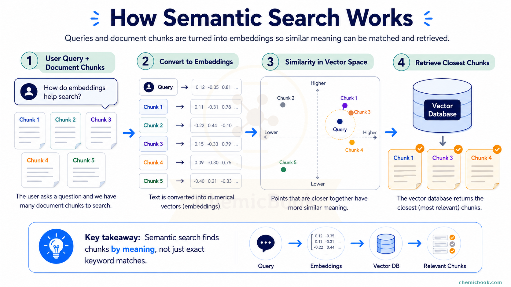
But how does embedding help in finding the relevant chunks? Here’s how:

1. We first embed all the chunks as well as the the user’s query into numerical vectors using an embedding model of our choice
2. Next, we compute cosine similarity between the user query vector with each of the chunks
3. Lastly, we can select one or more of the most similar chunks (highest cosine similarity) and pass them as the context

This process of finding the right chunks and using them as context is called Retrieval.

While we’re at the topic of Embeddings, let’s also talk about the Vector Databases.

Vector Databases

As the name indicates, these are specialized databases to store vectors (chunk embedding vectors in our case). Unlike traditional databases that primarily deal with structured data like text, numbers, and dates, vector databases are optimized for managing high-dimensional numerical vectors. While you don’t necessarily need to use them, they do offer some advantages.

1. Efficient Similarity Search: Vector databases are designed to quickly and efficiently perform similarity searches. In other words, vector databases streamline the computation of cosine similarity and finding top-k most similar chunks without having to write code for them.

2. Scalability and Performance: They are built to handle large volumes of high-dimensional vectors. Depending on the text, there can be millions of chunks and computing the similarity with each of them can take a long time. Vector databases use specialized indexing techniques like Approximate Nearest Neighbor (ANN) search, which significantly speeds up retrieval times compared to brute-force search methods.

Some examples of Vector Databases are Pinecone, Chroma, Qdrant, etc. All of them offer basic functionalities and, for most small use cases, it doesn’t really matter which one to use.

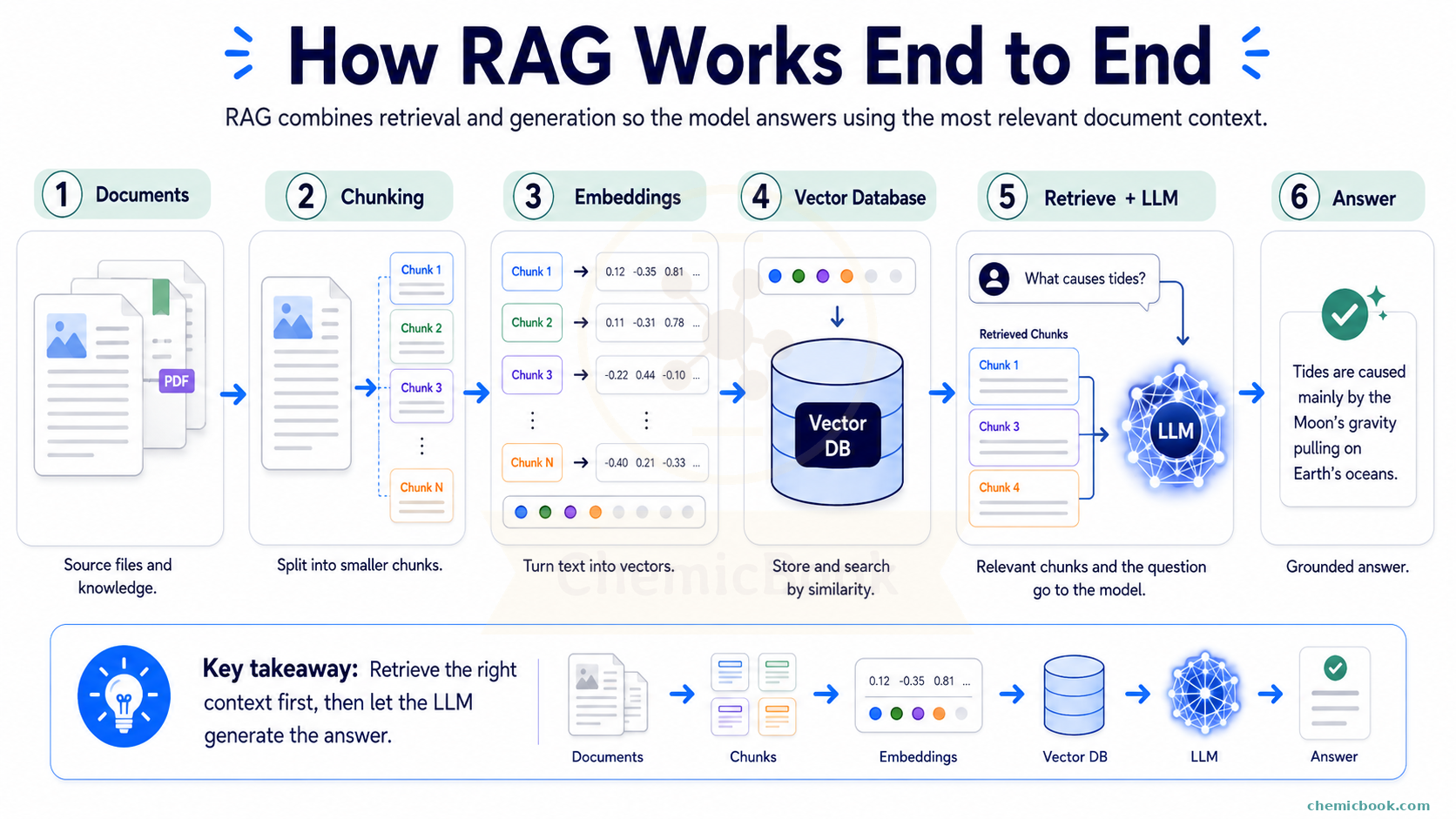
Wrapping up

Let’s quickly recap what we learned so far -  we wanted to ask questions about a book but due to context limit, we split it into chunks using any chunking method of our choice. To find the relevant chunks, we used embedding models to convert both chunks and the user query to numerical vectors and compute cosine similarity between them. We use the top-k most similar chunks as context. Lastly, to store vectors and make similarity search faster, we can use Vector Databases.

Tokens and Tokenization

Tokens

“GPT-4 has a context limit of 8000 tokens”

“Gemini 1.5 Pro has a context window of 1 million tokens”

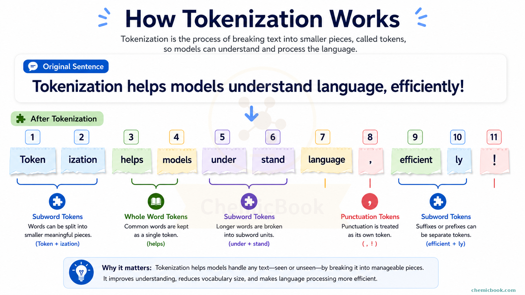
In these statements, what do you think is the meaning of the word “token”. If you’re thinking a token is equivalent to a word, you’re only partially correct. Tokens are the fundamental unit, the atom of Large Language Models. A token can be a word, a subword, a character, or even a punctuation. For example, in the sentence “Hello World!”, the tokens could be [“Hello”, “World”, “!”]. However, many modern models like ChatGPT use subword tokenization, where words are broken down into smaller units to handle rare words and different languages more efficiently. For instance, the word “unhappiness” might be tokenized as [“un”, “happiness”].

Vocabulary

The vocabulary of an LLM is a set of all unique tokens that the model can recognize and generate. It’s like the model’s dictionary. For instance, if a model has a vocabulary size of 50,000, it means there are 50,000 unique tokens that it understands.

The choice of vocabulary size is a critical design decision. A larger vocabulary allows the model to understand and generate more diverse and specific tokens, potentially improving its performance on a wider range of texts. However, it also increases the model’s complexity and computational requirements. Conversely, a smaller vocabulary can make the model faster and more efficient but might reduce its ability to handle rare words and nuanced language.

Further, each token in the vocabulary is indexed, meaning each token is assigned a unique number, like a label. For example, the word “hello” might be labeled as number 1, “world” as number 2, and so on. When the model works with text, it uses these numbers instead of the words themselves.

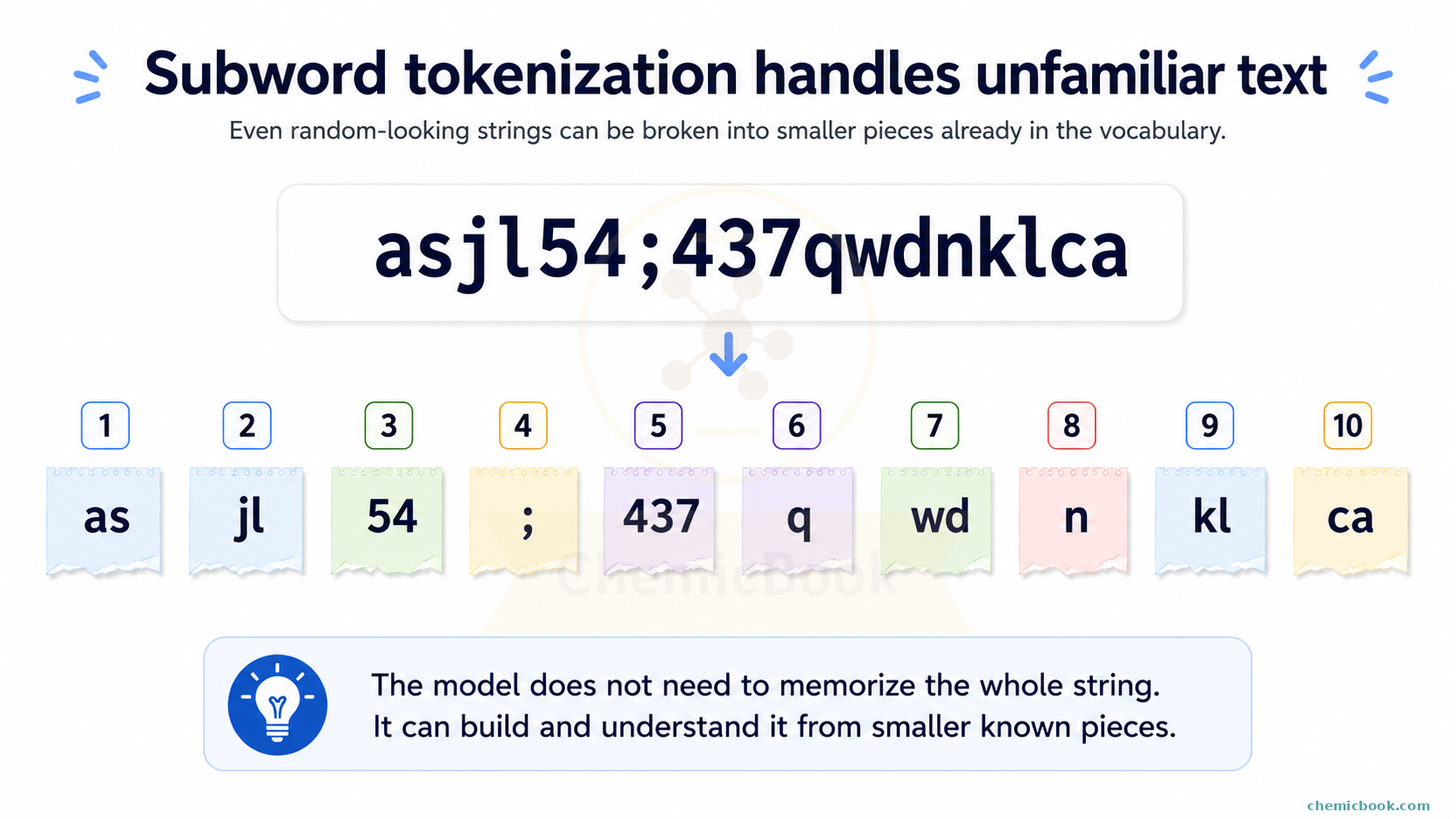
So if the model can only generate the tokens that are part of the vocabulary, then here’s a question for you: how come ChatGPT is able to generate the below answer correctly if the model has never seen the text “asjl54;437qwdnklca”? Take a minute to think about it. The next section will try to answer this question for you.

Tokenization

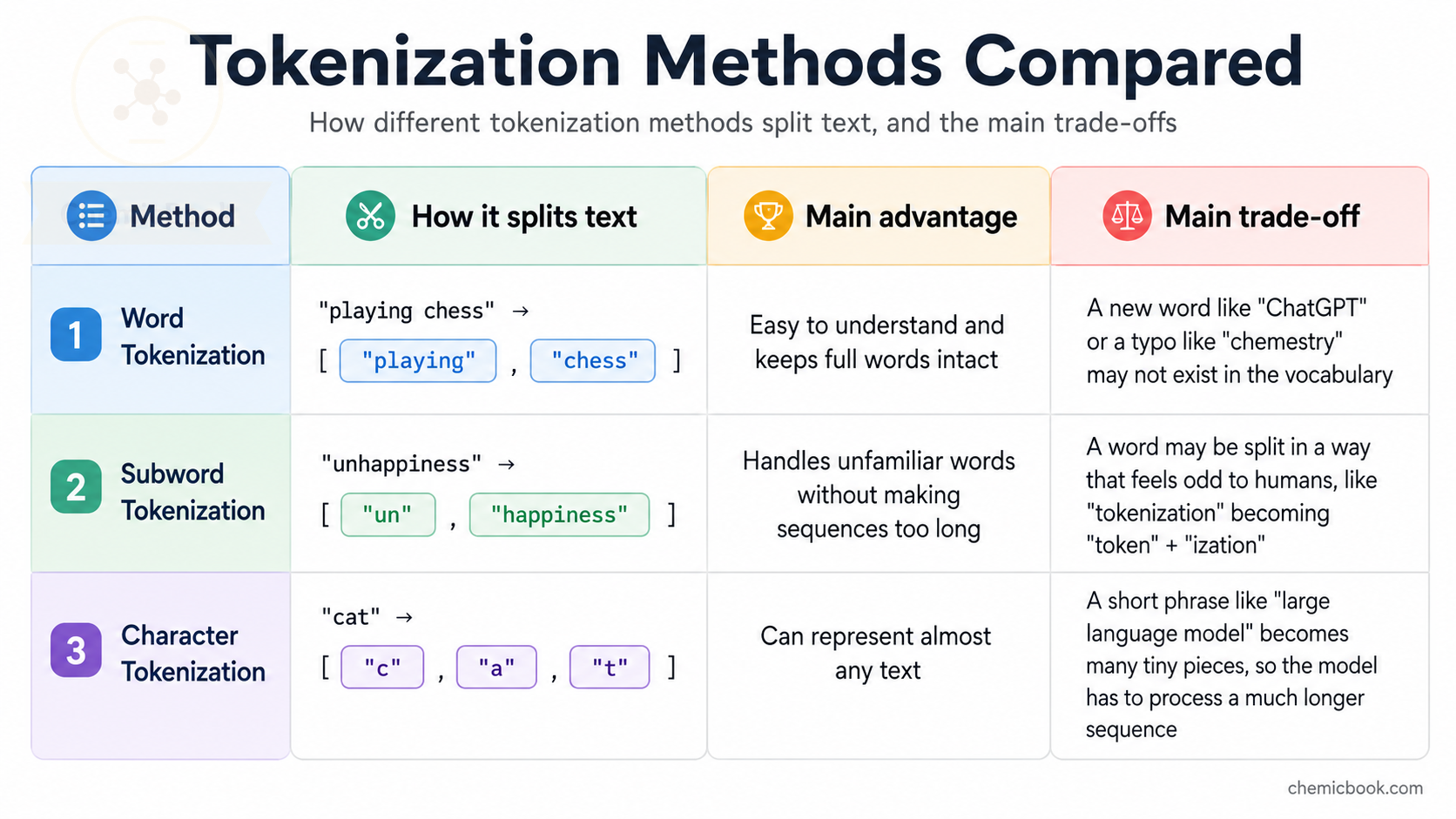
Tokenization is the process of translating strings (i.e. text) into sequences of tokens. Below are some most commonly used tokenization methods.

1. Word Tokenization: Splits text into individual words based on spaces and punctuation. Simple but can be inefficient for rare words and languages with complex morphology.
2. Subword Tokenization: Breaks words into smaller units (subwords) based on frequency and patterns in the language. Efficient for handling rare and out-of-vocabulary words.
3. Character Tokenization: Splits text into individual characters. Provides fine-grained control but can be computationally expensive and less efficient for capturing meaning.

As the below table shows, each method has a trade-off. Word tokenization is easy to understand, but it struggles with rare or new words because every word needs to exist in the vocabulary. Character tokenization can represent almost any text, but it makes sequences very long. Subword tokenization sits in the middle: it can handle unfamiliar words by breaking them into smaller known pieces, while still keeping the sequence shorter than character-level tokenization. This is why many modern LLMs use subword-based tokenization methods.

Here’s a quick comparison:

Coming back to the question I asked earlier, how can ChatGPT generate a text like “asjl54;437qwdnklca” even if it has never seen it before? The answer lies in the power of subword tokenization. The tokenizer first breaks the text into smaller pieces that already exist in the model’s vocabulary. This process is why even seemingly random or unfamiliar text can still be generated and understood by the model. For instance, the text “asjl54;437qwdnklca” might be broken down by GPT-4 into smaller units as shown below.

You can visit this link and play around with some combination of words to see it yourself.

Question for you: How many unique tokens are there in the below string? Head to the above link and see for yourself.

the the The
The THE
THE

LLM Finetuning Terminology

Parameter-Efficient Fine-Tuning (PEFT)

LLMs like GPT are generally good at understanding and generating text based on general knowledge. However, what if we want to make this model an expert in a specific domain, such as answering medical queries? To achieve this, we need to fine-tune the model using a specialized medical dataset.

Let’s take a simple example. Imagine we have already trained an LLM model and for simplicity, let’s assume there’s only one weight matrix (𝑊) in the model. You enter some input text, the model converts it to tokens, then to embeddings, perform some computation and generates an output. When a new specialized data is presented, we can train this model further (called fine-tuning) on this new data hoping that the LLM will learn the medical knowledge. However, there’s an issue: What if the model starts to overwrite its existing knowledge with the new information, potentially forgetting how to perform general tasks it was originally trained for? For example, while training the model to become an expert in medical knowledge, what if it starts forgetting how to understand and perform non-medical tasks? Afterall, a good doctor should have knowledge of the rest of the world too. This issue is called catastrophic forgetting.

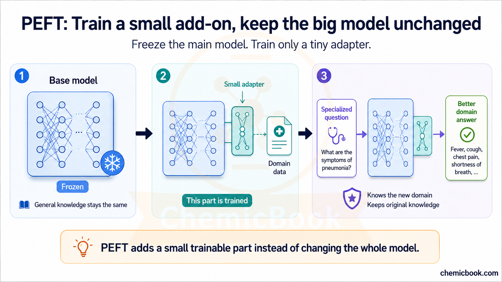
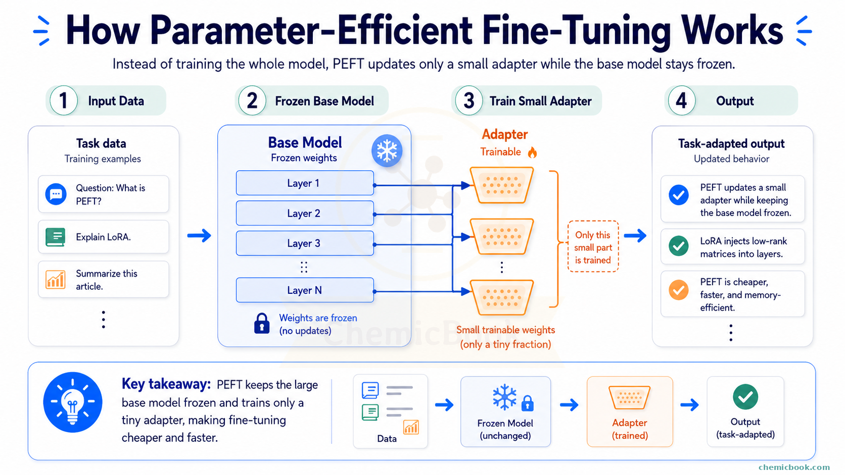
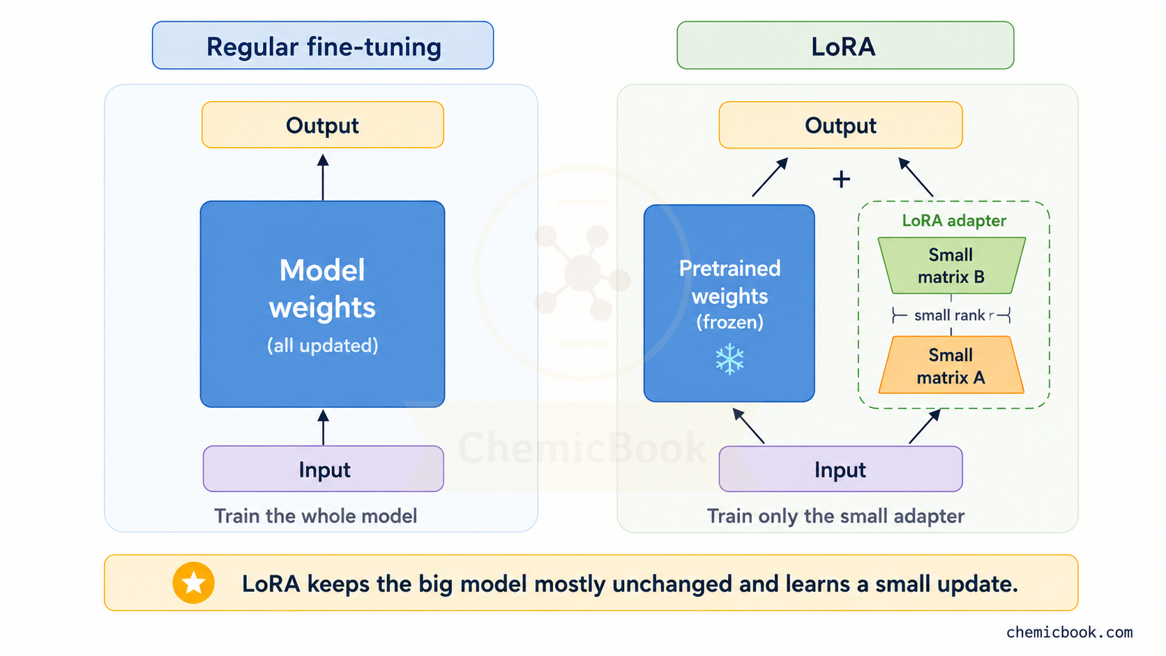
The solution here is PEFT: It addresses this problem by freezing most of the pre-trained model and training only a small number of additional or selected parameters, which makes fine-tuning cheaper and can reduce the risk of overwriting the model’s existing behavior. Here’s how it works:

1. Freezing the Original Weights: The original weight matrix 𝑊 is frozen, meaning its values are not updated during the fine-tuning process. This ensures that the general knowledge the model has acquired remains intact.
2. Adding Small Trainable Weights: Instead of changing the original matrix 𝑊, we add a much smaller set of new weights. These new weights are trained on the specialized dataset while the original weights stay frozen.
3. Training on New Data: When new data is passed through the model, it uses both the frozen weight matrix 𝑊 and the new small trainable weights. Since 𝑊 is frozen, its values are not changed. However, the new weights are updated during training, allowing them to learn the new information.
4. Final Output: Lastly, the new weights either modify or augment the existing model’s output. This way, the model retains its general knowledge while also incorporating the new, specialized information.

To summarize, PEFT adds a small number of new trainable weights while keeping most of the original model weights unchanged. These new weights learn the specialized information from the new dataset, and during generation they modify or guide the model’s output. This allows the model to adapt to a domain like medicine with much lower training cost, while reducing the risk of overwriting the general knowledge learned during pre-training. When a user asks a medical question, such as “What are the symptoms of diabetes?”, the model can use both its general language understanding and the task-specific adjustments learned during fine-tuning to produce a more relevant answer.

Low-Rank Adaptation (LoRA)

The Problem

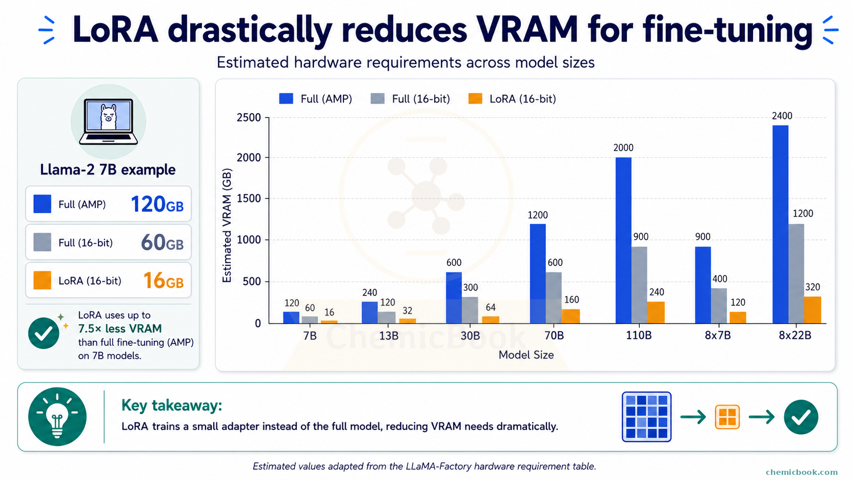
If you want to finetune an open-source model like Llama-2, say, on your laptop, you’re faced with the challenge of hardware requirements. You would typically need a minimum of 60 GB VRAM to finetune the Llama-2-7b model (the smallest of the models in Llama 2 family) with 16 bit precision. The requirement doubles to 120 GB if you use Automatic Mixed Precision (AMP), a technique that dynamically switches between 16-bit (half-precision) and 32-bit (single-precision) computations to optimize memory usage and speed. Below chart, borrowed from here, shows estimated hardware requirements for different models.

If you’re not familiar with what 32 bits and 16 bits precision mean, I’ll cover them in a separate blog post. For now, think of them as different levels of numerical precision that impact the speed and memory usage of your training process. In other words, using 16-bit precision allows you to fit larger models into the same amount of GPU memory, but at the potential cost of reduced numerical accuracy. On the other hand, 32-bit potentially ensures high accuracy but at the expense of increased computational demands. For many applications, this trade-off is worthwhile as it enables training models on more accessible hardware.

The Solution

Low-Rank Adaptation (LoRA) is an innovative approach that mitigates these hardware requirements by reducing the number of parameters needing finetuning. To understand LoRA, let’s first do a small exercise.

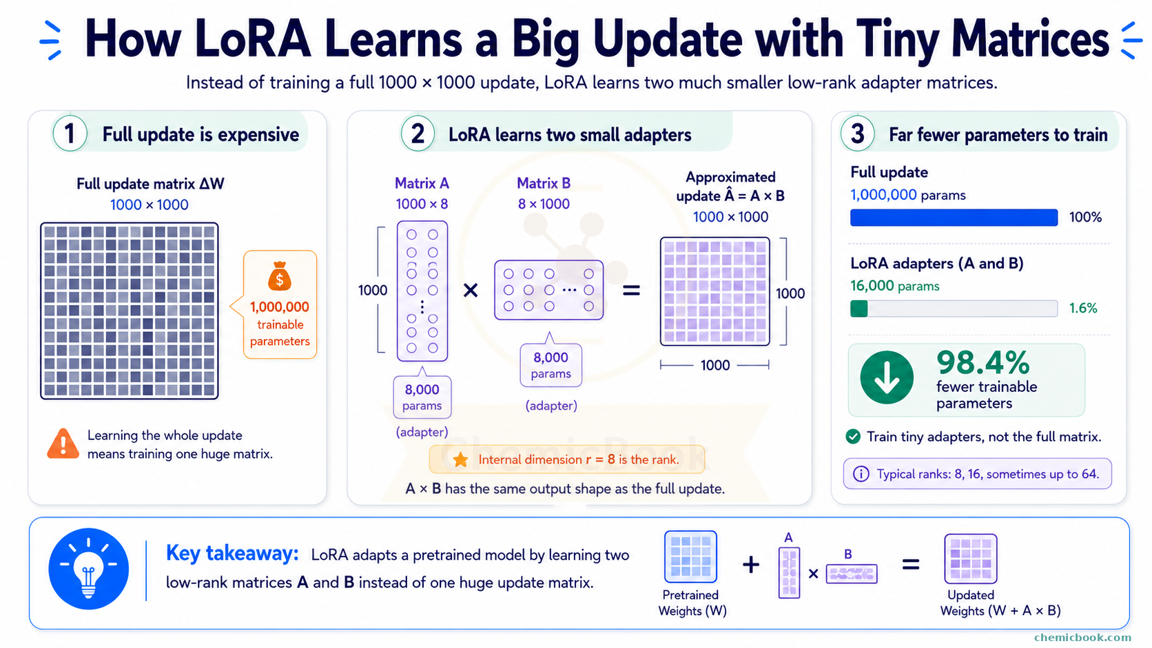
Let’s assume that the weight matrix, 𝑊, we saw in the PEFT section, has dimensions of 1000 x 1000. If we wanted to learn a full update for this matrix, that update would also need the same dimension. This means there would be 1,000,000 values (1 million parameters) that we would need to finetune.

Now let’s take two smaller matrices:

• 𝐴 (dimension 1000 x 8) - 8000 parameters and
• 𝐵 (dimension 8 x 1000) - again 8000 parameters
• Total combined 16,000 parameters

If you recall a matrix property from your school days: If you multiply two matrices - 𝐴 (dimension m x r) and 𝐵 (dimension r x n), the dimension of the new matrix will be m x n. So if we multiply 𝐴 and 𝐵 above, we’ll get a 1000 x 1000 matrix, which is the same size as the full update we wanted. Knowing this, what if we learn two smaller matrices 𝐴 and 𝐵 instead of learning one huge update matrix directly? This way, we only have to finetune 16,000 parameters compared to the original 1 million and if we multiply 𝐴 and 𝐵, we’ll get the same dimension as 𝑊. This is exactly what LoRA does. By learning two low-rank matrices instead of one large matrix, it reduces the number of trainable parameters by more than 98%, thereby lowering the computational cost. The mathematical idea behind LoRA is that low-rank approximations can capture the most important variations in the data with fewer parameters.

The internal dimension, r (in above example 8) is called the rank of the matrix. Usually, a rank of 8 or 16 is sufficient without sacrificing too much accuracy, however some tasks might require up to 64. The matrices 𝐴 and 𝐵 are called adaptors as they adapt the pre-trained model to new tasks by making minimal, yet effective changes.

Here’s a question for you: If LoRA is so effective in reducing computational requirements, is LoRA a one-stop solution for all finetuning tasks?

As the saying goes, there are no free lunches. In this case, there’s a trade-off between accuracy and computational power. While LoRA may reproduce a matrix of original dimension, 1 million parameters will likely capture a lot more information than 16,000 parameters. This raises the topic of Generalization vs. Specialization. Remember, the pretrained models like Llama are trained on many different types of dataset (generalized model) but by finetuning, we’re trying to make the model specialized for one task while avoiding the issue of catastrophic forgetting.

So here’s another question for you: If the parameter count is roughly the same, in fact we have added more parameters to the original base LLM, how does requirement reduces during fine-tuning? I mean for training, we still need to load the original model in memory for finetuning, right?

The answer is Yes, we do. We’ll still need to load the entire model in memory during finetuning too. However, there’s an additional component that you might not be familiar with. While training, additional RAM is required to compute the gradients and optimizer states and larger the weight matrix, higher the memory requirement to store gradients and optimizer states. Since, in PEFT and LoRA, we freeze the original weight matrices, gradients are not computed for them hence no additional RAM is required for them. And since our newly introduced matrices are much smaller in size, the corresponding gradient and optimizer states will also be smaller in size. When I said 60 GB of RAM is required for full-finetuning of Llama-7b model, this 60 GB also includes the RAM requirement for gradients and other training steps.

In case there’s still confusion, here’s a step-by-step explanation:

• Let’s say 60 GB RAM is required for full finetuning the Llama-7b model, assuming 16 bit precision. This includes around 14 GB (Llama-7b model size) to load the model in memory and remaining for the training steps like gradient computation
• During inference, we’ll only need around 14 GB of RAM (plus some additional requirement for loading the data and other processes) since training is done, so no more gradients
• When using LoRA, gradients are not computed for the frozen layers so we will need 14 GB to load the original model plus a few additional GBs depending on the rank of the matrices to load the smaller matrices plus some more RAM for their gradient and optimizer state computations. Typically, it goes around 16 GB total
• Lastly, during inference for the finetuned model, once again 14 GB to load the original model plus maybe 1 or 2 GB for loading the adaptors, depending on the rank. Let’s call it 16 GB just as an example

How can this requirement be brought down further? We can use a technique called Quantization.

Quantization

So far, we have talked about reducing the number of weights that need to be trained. Quantization takes a different approach. Instead of reducing the number of weights, it reduces how much memory each weight takes.

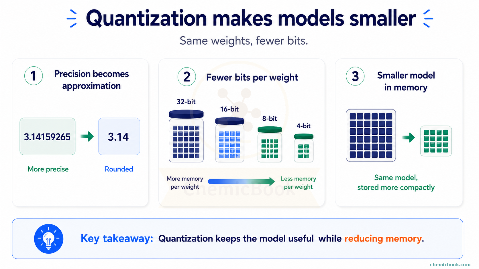
Let’s go back to a very simple example. Suppose we want to store the number:

3.14159265

If we store this number very precisely, we need more memory. But what if we store it as:

3.14

We lose a little bit of precision, but for many practical cases, this rounded value is good enough. Quantization follows a similar idea. It stores the model weights using fewer bits.

For example:

• In 32-bit precision, each weight uses 32 bits of memory
• In 16-bit precision, each weight uses 16 bits of memory
• In 8-bit quantization, each weight uses around 8 bits of memory
• In 4-bit quantization, each weight uses around 4 bits of memory

This means that if a model takes around 14 GB in 16-bit precision, a 4-bit version of the same model might take much less memory. The exact number depends on the quantization method and the framework being used, but the main idea is simple: fewer bits per weight means less memory.

A small intuition

Imagine you are storing someone’s height. If you write:

175.238492 cm

you are being very precise. But in most cases, writing:

175 cm

is enough. You have compressed the information. You lost some detail, but you kept the useful part.

Quantization does something similar with model weights. The model does not always need every tiny decimal detail of every weight to generate useful answers. By storing approximate values, we can make the model smaller and faster.

Why does quantization help?

Quantization is useful for both inference and fine-tuning.

During inference, quantization helps because the model takes less memory. This means we can run larger models on smaller GPUs or even on consumer laptops in some cases. It can also make generation faster because less data needs to be moved around in memory.

During fine-tuning, quantization can help because the frozen base model can be loaded in a lower-precision format. Then we only train a small number of additional weights, like the LoRA matrices we discussed earlier.

This brings us to a very popular technique called QLoRA.

Quantized Low-Rank Adaptation (QLoRA)

QLoRA combines the two ideas we just discussed:

1. Quantization: Load the original model in a lower-precision format, often 4-bit, to reduce memory usage.
2. LoRA: Add small trainable matrices and update only those during fine-tuning.

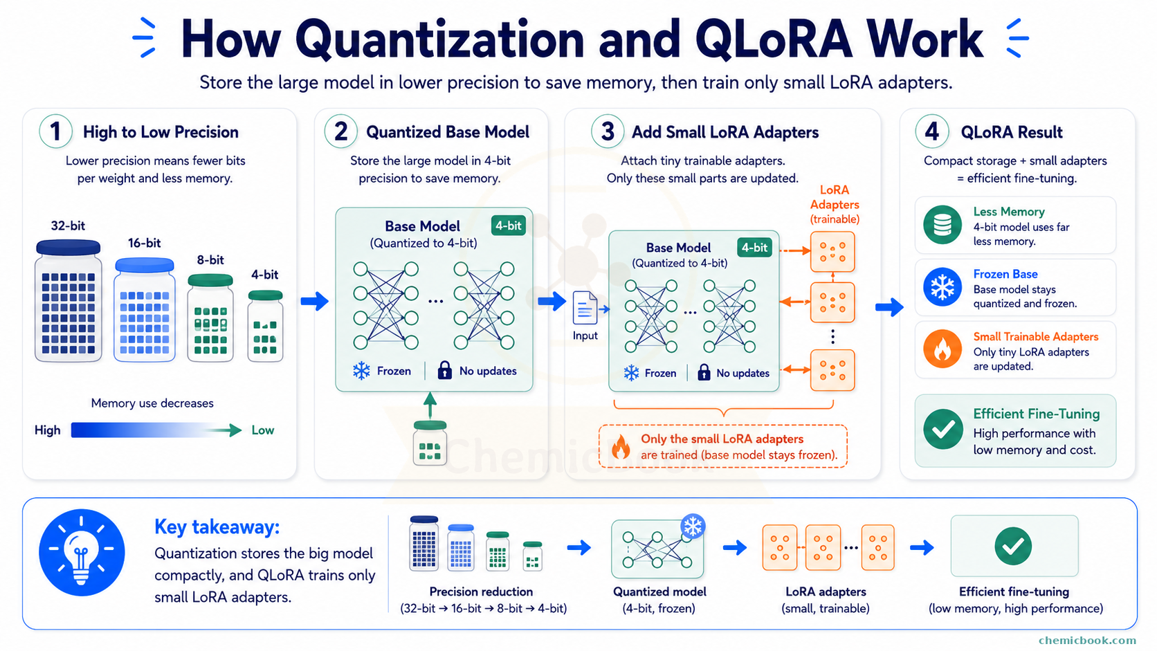
Let’s use our earlier Llama-7B example.

In normal LoRA fine-tuning, we still need to load the original model in memory. If the model is loaded in 16-bit precision, that alone can take around 14 GB. Then we need some extra memory for LoRA weights, gradients, optimizer states, and training data.

In QLoRA, the original model is loaded in 4-bit precision. So the base model takes much less memory. However, we do not train the 4-bit base model directly. The base model stays frozen, and we train only the small LoRA weights. This is why QLoRA makes it possible to fine-tune fairly large models on much smaller hardware.

Here’s the rough idea:

• Full fine-tuning: update almost all model weights
• LoRA: freeze the model and train small low-rank matrices
• QLoRA: load the frozen model in 4-bit precision and train small low-rank matrices

So if full fine-tuning is like renovating an entire building, LoRA is like adding a small extension to the building, and QLoRA is like doing that while storing the original blueprint in a compressed format.

Does quantization reduce quality?

Sometimes, yes. Since quantization stores approximate values, the model can lose some accuracy. But good quantization methods try to reduce memory while preserving most of the model’s performance.

The trade-off looks something like this:

• Lower precision means lower memory usage
• Lower memory usage means cheaper and more accessible training/inference
• But very low precision can sometimes reduce answer quality

For many practical use cases, 8-bit or 4-bit quantized models work surprisingly well. But if the task is very sensitive, such as medical diagnosis, legal reasoning, or scientific calculations, we should evaluate the quantized model carefully before trusting it.

Quantization vs LoRA vs QLoRA

Let’s quickly compare the three ideas:

Final Wrap-up

Let’s connect everything we learned.

We started with RAG, where we do not change the model at all. Instead, we retrieve useful information from an external source and pass it as context. This is useful when we want the model to answer using a document, a book, a website, or a private knowledge base.

Then we discussed tokens and tokenization, where text is broken into smaller units that the model can understand. Tokens are important because context length, input cost, and output cost are all measured in tokens.

Next, we looked at fine-tuning, where we actually update the model so it becomes better at a specific task or style. Full fine-tuning can be expensive because it updates many weights and requires a lot of GPU memory.

To make fine-tuning cheaper, we discussed PEFT, where most of the model is frozen and only a small number of parameters are trained. LoRA is one popular PEFT method that uses small low-rank matrices to learn task-specific changes. Finally, quantization reduces memory by storing model weights with fewer bits, and QLoRA combines quantization with LoRA to make large-model fine-tuning more practical.

So, at a high level:

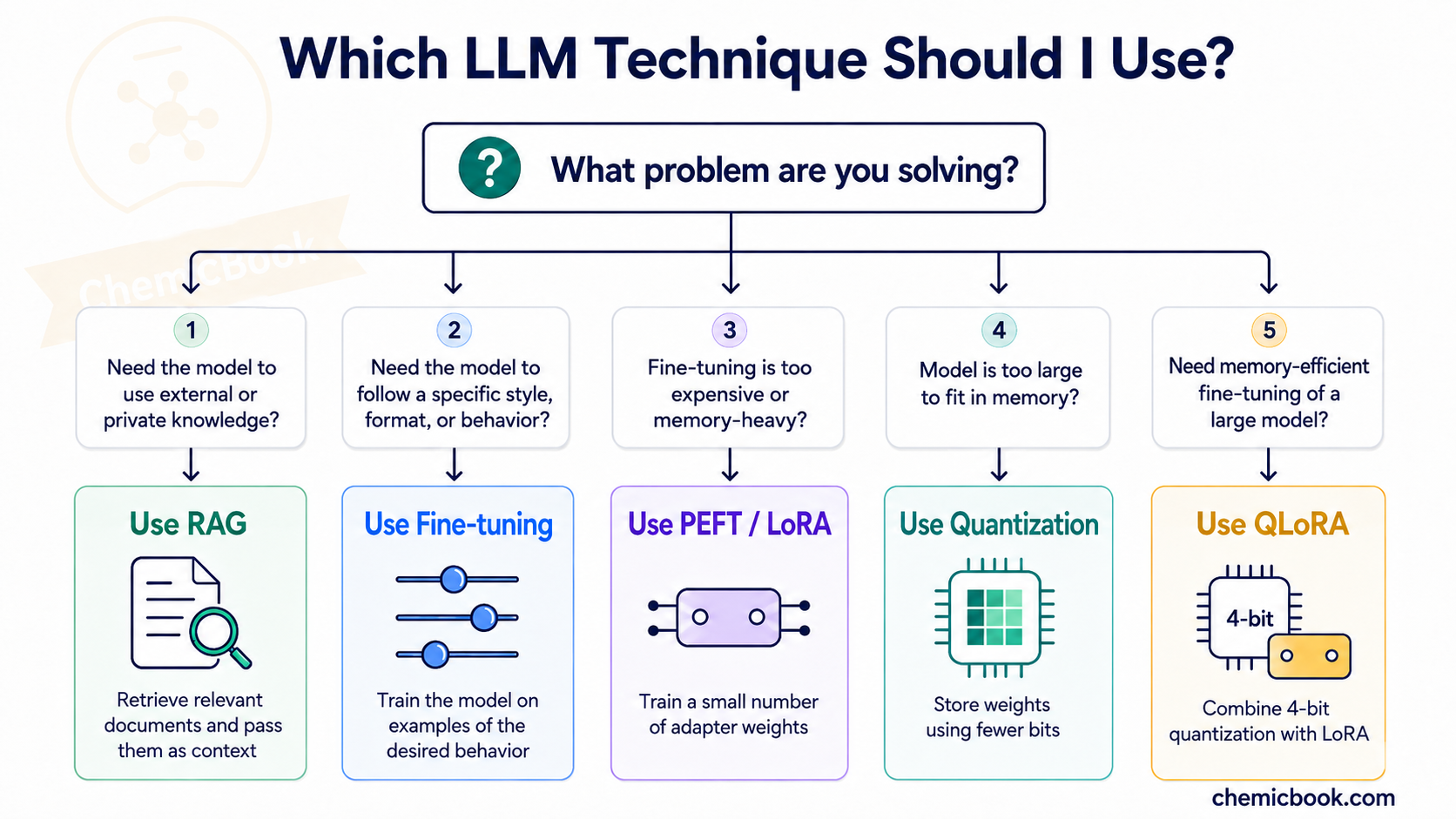
These are foundational ideas behind many modern LLM applications. Once these concepts are clear, topics like agents, tool calling, model serving, evaluation, and domain-specific AI systems become much easier to understand.